
Let’s consider a regular rectangular grid with step h on all axis.
Then as an approximation of, for instance, partial derivative  in the node j we can get the «finite difference»

where uj and uj-1 are the values of the unknown function u in horizontal neighboring nodes.
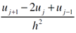
The approximation of a second order derivative  is naturally get as a difference of two «finite differences»
in the nodes j+1 and j, and divide it on h. Thus, we get the expression
is naturally get as a difference of two «finite differences»
in the nodes j+1 and j, and divide it on h. Thus, we get the expression
As a result, if we replace a derivative expression of PDE in each point of the grid to corresponding finite difference expression (for first and second derivatives), then we obtain the system of linear equations for the vector u = (uj)j=1,…,N, where N – is the number of nodes in the grid.
If this grid is big enough (it can have some millions, and even some billions of nodes, if the geometric region, where we are looking for a solution, is complicated enough), then the matrix of the system might have millions (or even billions) of rows and columns.
What helps in this situation (though the situation remains difficult enough), is that matrix of this system is very sparse (both by rows and columns).
The reason of sparsity is that while calculating derivatives we use only neighboring nodes of a grid, and there are very few neighbors – in one-dimensional grid there are only two neighbors, in two-dimensional grid there are only four neighbors, in three-dimensional grid – only six neighbors.
Thus, for a matrix that we have for rectangular grid in one-dimensional case we have not more than three non-zero elements in each row and column. For two-dimensional case grid matrix has not more than five non-zero elements in each row and column. And for three-dimensional grid – matrix has not more than seven non-zero elements in each row and column.
For more details on how the matrix looks like for elliptic problems go to this page.